客户端码农学习ML —— 逻辑回归分类算法
分类问题
在线性回归中,预测的是连续值,而在分类问题中,预测的是离散值,预测的结果是特征属于哪个类别以及概率,比如是否垃圾邮件、肿瘤是良性还是恶性、根据花瓣大小判断哪种花,一般从最简单的二元分类开始,通常将一种类别表示为1,另一种类别表示为0。
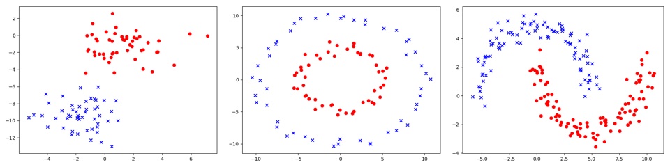
如下图,分别是几种不同的分类样式:
分类方法
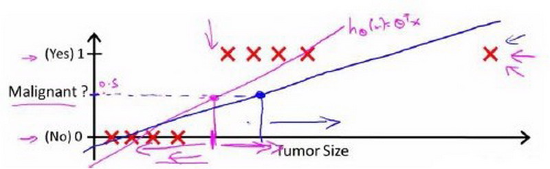
如果我们用线性回归算法来解决一个分类问题,那么假设函数的输出值可能远大于1,或者远小于0,会导致吴恩达机器学习教程中提到的分类不准或者阈值难以选择问题。
数学家们脑袋一转,想出来著名的sigmoid function,又名S形函数,是机器学习中诸多算法常用的一种激活函数,其图形如:
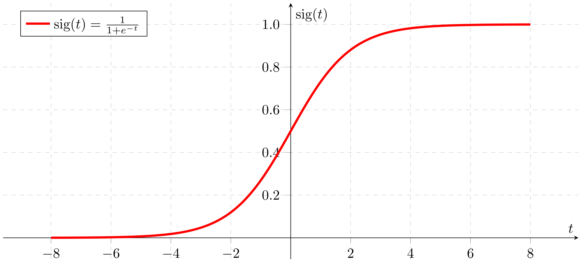
输出始终在0-1之间,完美应用在二分类问题,同时还能给出预测的概率。
将线性回归的输出应用sigmoid函数后,即得到逻辑回归的模型函数,又名假设函数Hypothesis:
【如果看到公式是乱七八糟的字符,请刷新下网页】
$$h_\theta(x) = g(\theta^T x) = \frac{1}{1 + e ^ {-\theta^T x}}$$
损失函数
在线性回归中,一般采用样本误差的平方和来计算损失,批量训练中求均方误差MSE或者均方根误差RMSE,此方法的损失函数是凸函数,我们通过遍历待定系数w画图形或者数学计算可证明。凸函数便于通过梯度下降法求出最优解。在一个特征下损失函数形如抛物线, 如下图中左边的子图:
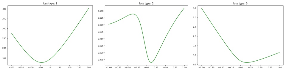
在加了sigmoid函数后,继续采用平方和来计算损失,得到的损失函数将不是个凸函数,难以求出全局最优解,图形绘制如上图中间的子图。
数学家们脑袋又一转,又想到了对数损失函数。
$$Cost(h_\theta(x),y)= \begin{cases}
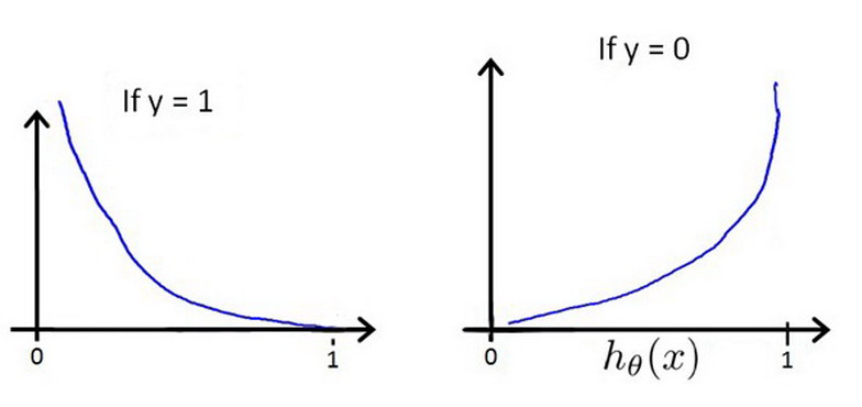
-log(h_\theta(x)) & \text{if $y$ = 1} \\
-log(1-h_\theta(x)) & \text{if $y$ = 0} \\
\end{cases}$$
当y=1时,图形形如下图中的左图,如果预测正确,损失为0,如果预测错误,损失无穷大。当y=0时,同样如果预测正确,损失为0,如果预测错误,损失无穷大。
写成一个完整的函数后变成:
$$Cost(h_\theta(x),y) = -y_ilog(h_\theta(x))-(1-y_i)log(1-h_\theta(x))$$
这个复杂的函数对于自变量θ是一个凸函数,画出的图形可看上面绿色图形中右边的子图,数学证明可求证二阶导数非负,可参考:http://sofasofa.io/forum_main_post.php?postid=1000921
代码实现分类
绘制损失函数图形
就是上面的绿色线条的图,首先准备数据和工具方法
1 | import numpy as np |
定义计算代码,实现多种损失函数计算,为便于绘制图形,假设b是固定值,只考虑w1系数变化,代码中的w参数等同于上述原理公式中的θ
1 | loss_type = 3 |
绘制出图形
1 | if __name__ == '__main__': |
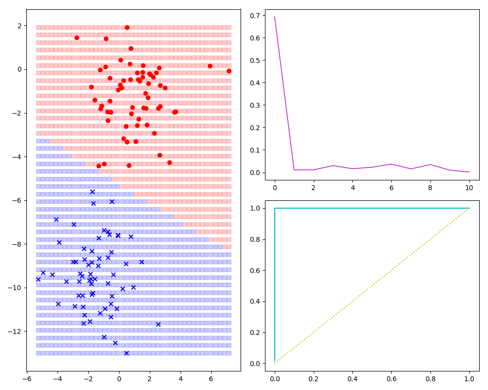
实现线性可分样本分类
即第一张图左边样本的分类,先给出完成效果看看:
导入库,生成mock数据,并定义h(θ)
1 | import numpy as np |
定义优化器、训练并打出最优超参数看看。
1 | use_base_method = 3 |
数据分类并模仿google的A Neural Network playground绘制分类背景:
1 | class1_x = [x[0] for i, x in enumerate(data) if target[i] == 1] |
工具方法如下:除绘制图形外,顺便输出了预测精度。
1 | import numpy as np |
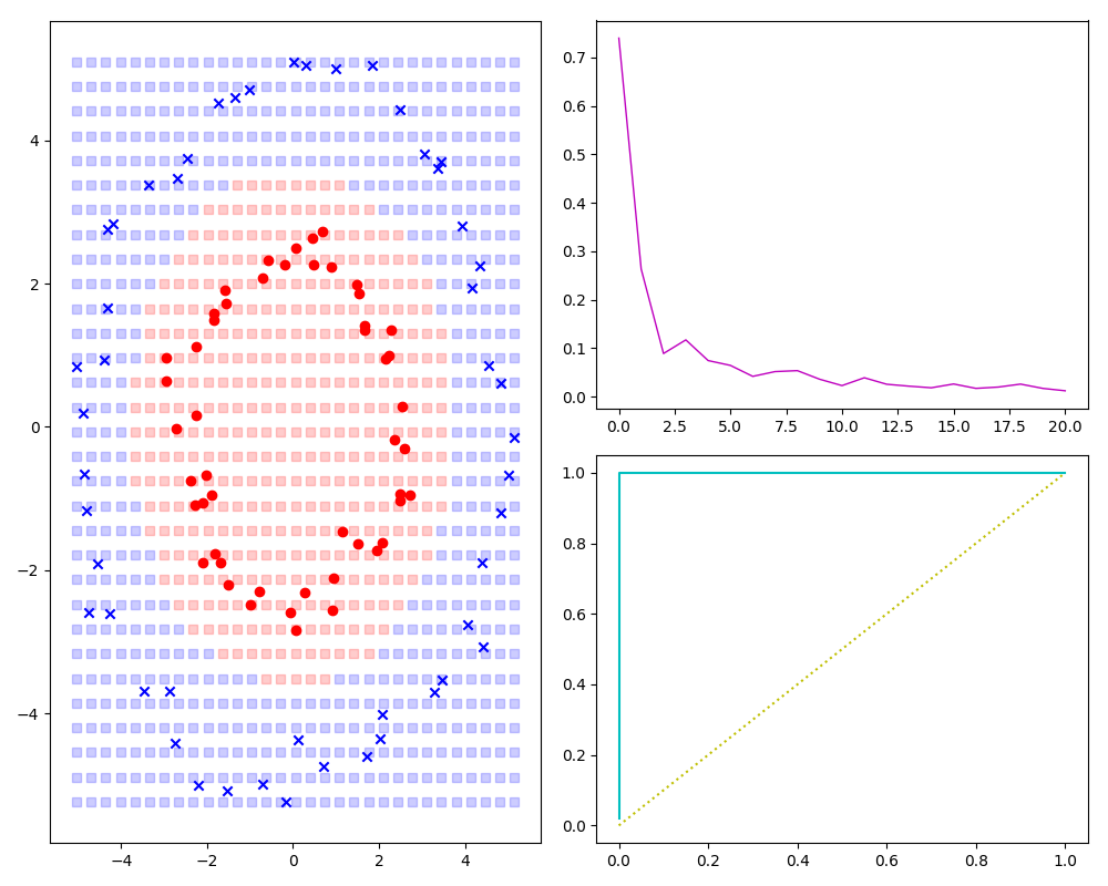
实现圆形分类的样本分类
相对于上述线性可分样本,主要有两点不同,一是样本生成,二是h(θ):
1 | # 样本生成: |
1 | # h(θ) result_matmul1 2的值改为平方后再乘以w系数 |
效果预览如下图:
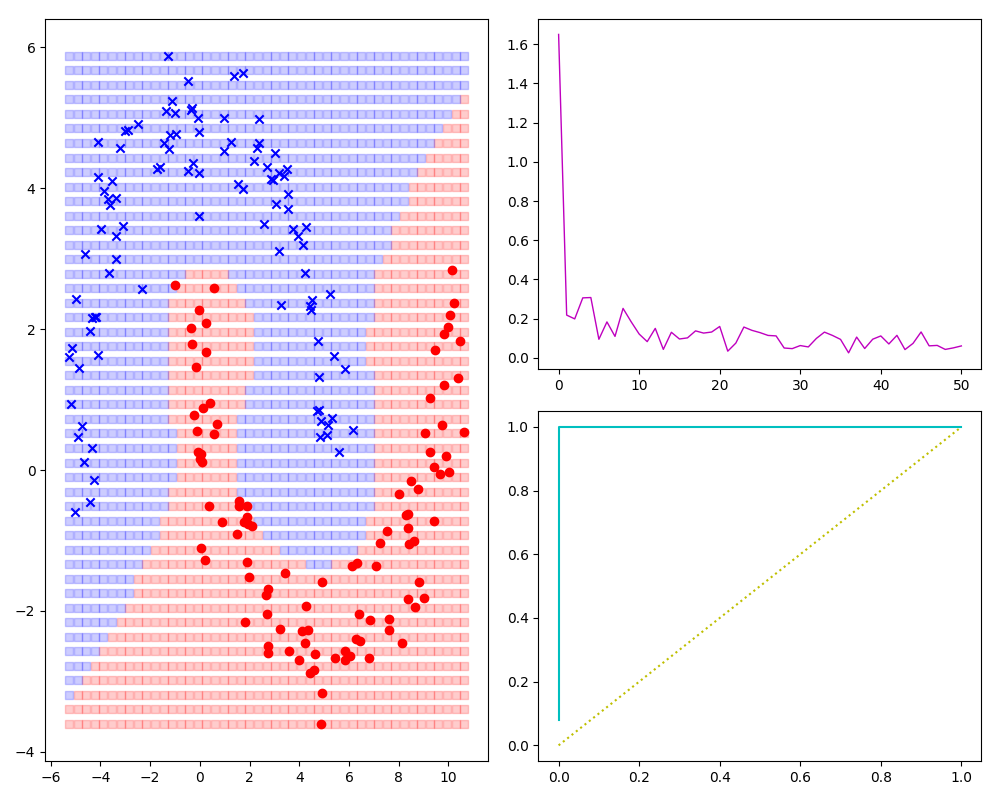
实现不规则分类的样本的分类
对于下图,一般不能立即看出什么假设函数能对应(数学高手或者有经验的除外),此时先用大杀器多项式多次试验,多项式写的够全、试验次数够多总能找到相对合适的模型。
1 | # 同样样本生成: |
1 | # 大量超参数定义 |
效果预览如下图:
参考:
http://sofasofa.io/forum_main_post.php?postid=1000921