客户端码农学习ML —— 使用LinearRegressor实现线性回归

最近看了Google官方机器学习教程,跟着练习了部分示例,其中《使用 TensorFlow 的起始步骤》采用了LinearRegressor配合Pandas来进行线性回归训练。

于是使用两者重新写了一个版本的线性回归训练,数据也从之前python直接生成模拟数据改成了从csv文件读取,而csv文件来源于Excel: A列的100行等于1至100的序列, B=A*5+50+RANDBETWEEN(-10, 10)。

读取数据集及特征准备

1
2
3
4
5
6
7
8
9
10
11
12
13
14
15
16
17
18
import numpy as np
import pandas as pd
from sklearn import metrics
import tensorflow as tf
from tensorflow.python.data import Dataset
import math

linear_dataframe = pd.read_csv("../data/linear_data.csv", sep=",")

print('linear_dataframe.describe()=%s\n' % linear_dataframe.describe())

x_series = linear_dataframe["x"].apply(lambda x: max(x, -10000))
my_feature_dataframe = linear_dataframe[["x"]]

x_feature_column = tf.feature_column.numeric_column("x")
feature_columns = [x_feature_column]

target_series = linear_dataframe["y"]

训练

1
2
3
4
5
6
7
8
9
10
11
12
13
14
15
16
17
18
19
20
my_optimizer = tf.train.GradientDescentOptimizer(learning_rate=0.0001)
# my_optimizer = tf.contrib.estimator.clip_gradients_by_norm(my_optimizer, 5.0)

linear_regressor = tf.estimator.LinearRegressor(feature_columns=feature_columns, optimizer=my_optimizer)


def my_input_fn(feature_dataframe, target_series, batch_size=1, shuffle=True, num_epochs=None):
features = {key: np.array(value) for key, value in dict(feature_dataframe).items()}

ds = Dataset.from_tensor_slices((features, target_series))
ds = ds.batch(batch_size).repeat(num_epochs)

if shuffle:
ds = ds.shuffle(buffer_size=10000)

features, labels = ds.make_one_shot_iterator().get_next()
return features, labels


_ = linear_regressor.train(input_fn=lambda: my_input_fn(my_feature_dataframe, target_series), steps=2000)

结果评估

1
2
3
4
5
6
7
8
9
10
11
12
13
14
15
16
17
18
19
20
21
22
23
24
25
26
27
28
29
predict_input_fn = lambda: my_input_fn(my_feature_dataframe, target_series, num_epochs=1, shuffle=False)
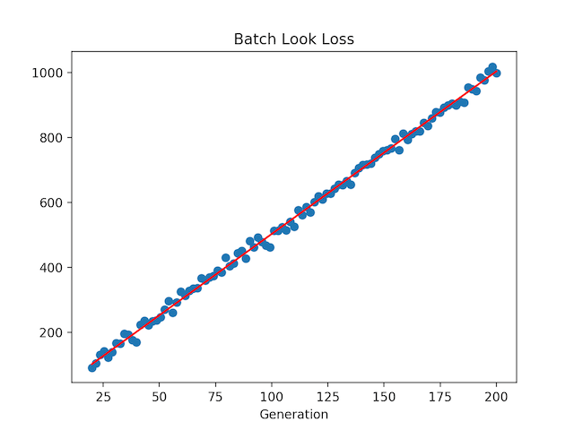
predictions = linear_regressor.predict(input_fn=predict_input_fn)
predictions = np.array([item['predictions'][0] for item in predictions])

mean_squared_error = metrics.mean_squared_error(predictions, target_series)
root_mean_squared_error = math.sqrt(mean_squared_error)
print("Mean Squared Error (on training data): %0.3f" % mean_squared_error)
print("Root Mean Squared Error (on training data): %0.3f" % root_mean_squared_error)

min_y_value = target_series.min()
max_y_value = target_series.max()
min_max_difference = max_y_value - min_y_value

print("Min. x Value: %0.3f" % min_y_value)
print("Max. x: %0.3f" % max_y_value)
print("Difference between Min. and Max.: %0.3f" % min_max_difference)
print("Root Mean Squared Error: %0.3f" % root_mean_squared_error)

weight = linear_regressor.get_variable_value('linear/linear_model/x/weights')
bias = linear_regressor.get_variable_value('linear/linear_model/bias_weights')
print('\n weight=%s bias=%s' % (weight, bias))
[[_w]] = weight
[_b] = bias

result_dataframe = pd.DataFrame()
result_dataframe["predictions"] = pd.Series(predictions)
result_dataframe["targets"] = target_series
print('\nresult dataframe:\n%s' % result_dataframe.describe())

结果可视化

1
2
3
4
5
6
7
8
9
10
11
12
13
14
15
16
17
18
19
20
21
22
def show_visualization_data(x_data_array, y_data_array, w, b, loss_vec, title=None):
best_fit = []
for x in x_data_array:
best_fit.append(w * x + b)

plt.figure()

if title is not None:
plt.title(title)

ax = plt.subplot(121)
ax.scatter(x_data_array, y_data_array, color='y', label="样本", linewidths=0.5)
ax.plot(x_data_array, best_fit, color='b', linewidth=2)

if loss_vec is not None:
ax = plt.subplot(122)
ax.plot(loss_vec, color='g', linewidth=1)
ax.set_ylim(0, 1000)

plt.show()

show_visualization_data(x_series, target_series, _w, _b, None, title='Pandas')

可以得到与上一篇《客户端码农学习ML —— 用TensorFlow实现线性回归算法》文中相似的图片:

ai_kai_line_only_mul_batch_line

参考

https://developers.google.cn/machine-learning/crash-course/prereqs-and-prework

https://colab.research.google.com/notebooks/mlcc/first_steps_with_tensor_flow.ipynb?hl=zh-cn


本文首发于钱凯凯的博客 : http://qianhk.com/2018/02/客户端码农学习ML-使用LinearRegressor实现线性回归/